

Hofstadter's Butterfly: Reconstructing a Fractal Energy Spectrum with GLSL in TouchDesigner
Real-time GLSL reconstruction of Hofstadter’s butterfly in TouchDesigner, analytical approximations, and the computational posture of attention.

A couple of months ago, I made an Instagram post with a short render of this project (basically filming my laptop screen with my phone), a real-time GLSL reconstruction of Hofstadter’s butterfly in TouchDesigner. At the time, I described it quickly, posted a couple of interesting sources about it on Stories, and left it there. I still haven’t made the time to properly render and output the visuals in a way that does justice to the intricacy of the system, but this article is, in a way, an attempt to return to what was behind it.
Honestly, I also wanted to write about why this subject, Hofstadter’s quantum physics butterfly, captivated me in the first place. Maybe part of the reason is that it already had this personal charge around it, because in recent years, I have encountered butterflies in a very particular way, always during equally particular moments in my life that I’d call phases of transition, moments when the previous reality had already collapsed, or was changing form, and I found myself forced to pay attention, to look more closely, to be present.
It was the Christmas and New Year period and Copenhagen was completely silent: everyone, including my colleagues, was shut inside with their families. I kept going to the office every day for the purpose of using a computer more powerful than my own. It was during those days that I deep-dived into the research and development of this small project. Inspired by the YouTube video Good News in 2025 (You Might Have Missed), I was reflecting on the progress and discoveries of 2025, looking for something that could make the end of the year feel special and positive. Among the files, images, and experiments I had collected, there was also this lab discovery successfully achieved in 2025: Hofstadter’s butterfly.
And alongside it, at the time there was also a broader question that I wanted to explore more in my work, such as how do you visualize something that does not exist in a directly perceptible space? The following screenshot is part of a big Obsidian canvas I was putting together at the time, and it was basically a moodboard around the ideas of the ineffable, attention, and being present, all the material that was orbiting around this question before it became a TouchDesigner and GLSL project.
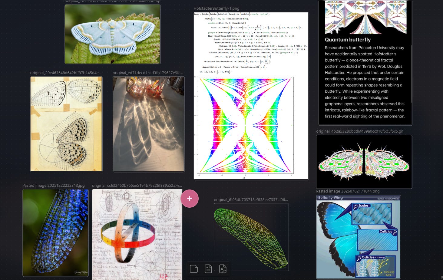
Months later, having moved across the world once again, I found myself thinking about those findings. Here, in Busan, Korea, I have been seeing many butterflies. Maybe because I am paying more attention, maybe because the city itself offers a more favorable natural environment; considering that it mostly happens when I walk along the river by the subway station, it is probably both. So, I decided to return to this project, developed in GLSL on TouchDesigner around New Year’s, by writing this article.
This is also a build log of the visualization of Hofstadter’s butterfly I made in TouchDesigner, which, for those unfamiliar with it, is a visual programming software used to create interactive systems, real-time visualizations, and audiovisual installations. The technical core is a GLSL compute shader (OpenGL Shading Language, a C-style language that executes directly on the GPU) that approximates spectral density in a plane of magnetic flux and energy, extracts the structure of the bands through finite differences, and instances oriented geometry with GLSLcopy POPs as a vector field
Before getting there, though, I want to talk about the concept itself: what Hofstadter’s butterfly is, why it is so wonderful, and how it appeared outside theory, outside books, in the laboratory for the first time in 2025 almost by chance, and, in a charming way, exactly as real butterflies do when you are truly paying attention.
1. Before the Build
1.1 What the butterfly is
Hofstadter’s butterfly is an energy spectrum. More precisely, it is a map of the possible energy levels of an electron moving on a two-dimensional lattice while being crossed by a perpendicular magnetic field.
Put like that, it might sound fairly abstract. But the point is that if we imagine the electron not as a tiny ball moving freely through space, but as a wave function that can exist only under certain precise conditions, then the energy spectrum becomes the drawing, the shape, of those conditions. It is the list, or rather, the geometry, of the energies the electron is allowed to occupy.
Douglas Hofstadter calculated it in 1976 for his doctoral thesis at the University of Oregon1. The surprising part of the thesis was the result consisting in a structure that keeps splitting into bands, sub-bands, and even smaller sub-bands, recursively. The shape looked like a butterfly because the mathematics of the system produced, symmetrically, a kind of numerical organism that changes according to the ratio between the magnetic field and the lattice.
In this sense, I am reminded of Jason Padgett2, an acquired savant who began perceiving the world through mathematical fractals after a brain injury, and of the way he insists that there is a fractal in literally everything. His figure and mathematical interpretations are debated, but what I find useful is the intuition that a deep rule can keep rewriting form through different scales. An intuition that, to me, both exceeds mathematics and is mathematics itself. I am also drawn to the way he talks about perception through waves, frames, frequencies, and relative positions, because it tackles the same question of what becomes visible when attention changes, which is what brought me to this project in the first place.
This butterfly, too, can be seen as quantum energy levels making a self-similar structure visible as a recursive pattern produced by the relation between magnetic flux, phase, and periodicity.
More concretely, we have to move from the image back to the mathematical model that produces it. In the Harper-Hofstadter model3, an electron moves on a two-dimensional square lattice, not freely, but by hopping between neighboring lattice sites. In the presence of a perpendicular magnetic field, the hopping is modified by a complex phase factor. This is the Peierls phase4.
The important quantity is the total phase accumulated around one closed cell of the lattice. That total phase is determined by the magnetic flux passing through the cell. In quantum mechanics, phase controls how waves interfere with one another, so changing the magnetic flux changes the way the possible paths of the electron combine.
1.2 From theory to measurement
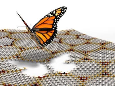
In the 1970s, Hofstadter’s butterfly was still a theoretical prediction and the problem was the physical scale. In ordinary materials, the distance between atoms is at the scale of angstroms, so pushing one flux quantum through a single lattice cell would need a magnetic field way beyond what a lab could possibly produce.
This is where moiré materials come in. When two lattices sit on top of each other with a slight rotation, they produce a larger interference pattern. The atomic lattice stays tiny, but the overlapping structure creates a new, much larger repeating cell: the moiré superlattice. The twist angle sets the scale of that repeating pattern. Particularly, in twisted bilayer graphene, two graphene layers get stacked with one layer slightly rotated relative to the other, and this produces a superlattice that can run much larger than the original graphene unit cell.
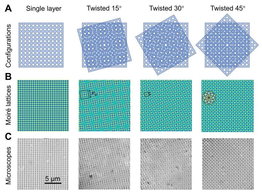
That larger cell is what makes Hofstadter physics reachable in a lab. Instead of pushing one flux quantum through an atomic-scale cell, the system effectively hands you a larger moiré cell to work with, and a larger cell means the same flux condition shows up at a much lower magnetic field.
So, now we get to 2025, a Princeton team led by Ali Yazdani was fabricating twisted bilayer graphene to study superconductivity, aiming for the magic angle of about 1.1°5. During the process of fabrication they undershot that angle, the sample actually came out closer to what’s now described as the second magic angle6, and the moiré pattern ended up with a longer periodicity than intended. That mistake was the whole story, as it turned out that a longer moiré period is exactly the condition needed to resolve Hofstadter’s subbands with scanning tunneling spectroscopy, which is a condition nobody had managed to hit on purpose.
That accident made the Hofstadter spectrum visible through direct spectroscopy, for the first time in fifty years. The image wasn’t the clean butterfly diagram people usually picture; it was experimental data, messier and more indirect than a simulation. What emerged, however, was the unmistakable signature of flat moiré bands splitting into Hofstadter subbands, mirroring the exact recursive logic that made the original 1976 prediction so deeply disruptive to physics at the time, revealing an infinitely fragmenting, jagged fractal where traditional quantum mechanics expected smooth, predictable states.
Nobody in that lab set out to find it but someone was paying close enough attention to recognize what they were looking at.
2. How fractions become form
2.1 Phase and repetition
Hofstadter starts from a problem in condensed matter physics: an electron moving in two dimensions inside a periodic potential, meaning a structure that repeats like the ideal lattice of a crystal. A perpendicular magnetic field is applied to this structure, and the result is a graph where the horizontal axis represents the magnetic flux passing through one cell of the lattice, while the vertical axis represents the energies allowed for the electron.
The flux per cell is written as Phi and it is measured relative to the flux quantum:
And the following ratio tells us how much of one flux quantum passes through each cell, which explains how the butterfly shows what happens to the energy spectrum as alpha changes:
In quantum mechanics, the electron is described by a wave function. When this wave function completes a closed loop around a cell crossed by a magnetic field, it accumulates a phase equal to:
The magnetic field changes the periodicity of the problem. The material lattice repeats cell after cell, but the wave function also has to remain compatible with the phase it accumulates along the path.
When alpha = p/q, this compatibility is recovered on a larger scale. After q cells, the total flux is p Phi_0, so the accumulated phase corresponds to an integer multiple of 2π. This is why the periodicity of the system returns only after q cells. In the standard square lattice model, this produces q subbands.
A simple way to picture this: imagine an arrow rotating by a fixed fraction of a full turn each time it moves to the next lattice site. If it rotates by 1/3 of a turn per step, it points in its original direction again after 3 steps. If it rotates by 1/5, it repeats after 5. The denominator q is that repeat length, it sets the scale at which periodicity, and with it the subband structure, becomes readable again.
The denominator q becomes a physical scale in the problem. It indicates the scale at which periodicity becomes readable again, and that scale determines how finely the spectrum fragments.
Irrational values can be understood as limits of sequences of rational numbers with larger and larger denominators. The periodicity is pushed further and further away. This passage to the limit is one of the reasons the butterfly becomes fractal.
At this level, it also makes sense to mention arithmetic structures such as the Farey sequence and the Stern-Brocot tree7. These are ways of organizing fractions between 0 and 1 according to their proximity and the size of their denominators. They become useful because the horizontal axis of the butterfly is exactly the ratio alpha = Phi/Phi_0.
If two rational values of the flux, p/q and p'/q', mark two nearby regions of the spectrum, an intermediate ratio can appear between them through the mediant:
This new fraction has a larger denominator, so it corresponds to a finer scale of the structure.
In the butterfly, this arithmetic helps us read why major regions contain smaller subregions, and why these subregions gather around increasingly precise fractions of the magnetic flux.
A full physical explanation would lead into the Harper-Hofstadter model and magnetic Bloch conditions, but the point I want to stay with is simpler: rational order becomes visible. Farey sequences and the Stern-Brocot tree work like coordinates for navigating the fractions that structure the horizontal axis.
2.2 The meaning of the gaps
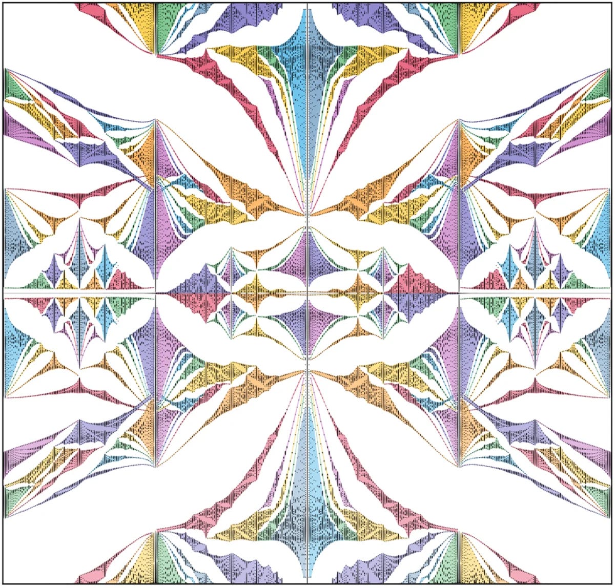
In the graph, empty-looking regions appear between the bands. Physically, the gaps are intervals of energy where no available electron states appear. They separate the bands, but they also have information about the system.
To describe them, physicists often use Wannier diagrams. These diagrams move the focus from energy to electronic filling. They ask how many states are occupied as the magnetic flux changes.
In this plane, the gaps follow a Diophantine relation between filling and flux:8
Here, s distinguishes the gap within the spectrum, while t is an integer connected to the quantized Hall conductivity9:
This means that a gap in the spectrum can correspond to a measurable electrical response.
The butterfly contains all of these layers in the same image. A continuous change in magnetic flux produces a structure organized by fractions, those fractions determine magnetic unit cells and subbands and the gaps mark forbidden energies and carry topological numbers connected to the Hall response.
The form of the butterfly comes from both the energies the electron can occupy, and the energies that remain excluded.
3. The visualization in TouchDesigner
To reconstruct the butterfly in TouchDesigner, I chose to build it as a field of points: a grid remapped into flux / energy coordinates, then passed through a GLSL shader that calculates density, color, scale, rotation, and rational hierarchy.
The main premise is that this is still a draft. I developed it by focusing mainly on the visualization rather than on a complete physical simulation of the Harper-Hofstadter model. The shader does not diagonalize matrices and does not calculate the spectrum rigorously. Instead, I used an analytical shortcut based on rational values p/q, light enough to run in real time and create a fast prototype.
The TD network is divided into four steps:
preparing a grid of points;
transforming it into
flux / energycoordinates;calculating density and visual attributes in GLSL;
instancing geometry over the field.
3.1 Grid and coordinates
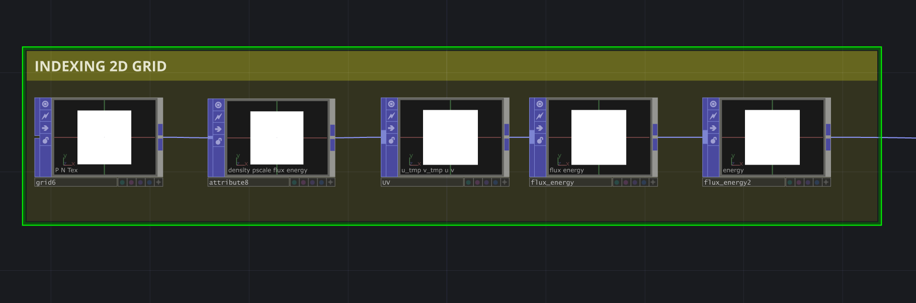
The network starts with a Grid POP of 200 columns and 200 rows, which is a resolution producing 40,000 points.
Right after that, an Attribute POP creates the custom attributes that will later be written by the shader: density, pscale, flux, energy.
The next step is to transform the grid into a flux / energy domain.
The Grid POP produces a linear sequence of points, from 0 to 39999. To use it as a two-dimensional plane, I derive two normalized coordinates from _PointI:
u_tmp = _PointI mod 200
v_tmp = _PointI / 200
u_tmp corresponds to the horizontal position of the point in the grid, while v_tmp corresponds to the vertical progression. Both are then normalized:
u = u_tmp / 199
v = v_tmp / 199
This way, every point receives u/v coordinates between 0 and 1, independent of the geometric size of the grid. After this normalization, u is used as flux, while v is centered and scaled to obtain energy:
flux = u
energy = (v - 0.5) * 5
The result is a stable parametric plane where flux goes from 0 to 1, and energy goes from about -2.5 to 2.5.
3.2 The first shader: building the butterfly field
3.3 glsl_FIELD
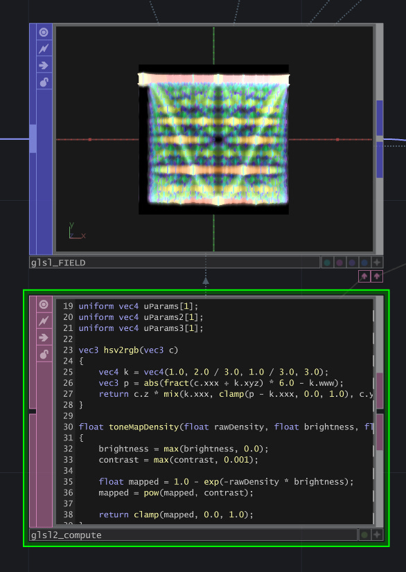
glsl_FIELD is the first shader where the project really starts to become the butterfly.
Before this point, the network is still preparing the grid. Each point has a position, and after the remapping step each point also has two values attached to it:
flux
energy
These are the two coordinates of the butterfly. flux tells the shader where the point is on the horizontal axis, and energy tells it where the point is on the vertical axis.
So, for every point in the grid, the shader asks: at this flux, and at this energy, how much of the butterfly is present?
That value becomes density.
If a point is close to one of the approximated bands, its density increases. If it falls in a gap, or in an area where no band is being strongly approximated, its density stays low.
The same shader also prepares the attributes used later by the instancing system:
P
P_flat
density
pscale
Color
RotX, RotY, RotZ
gmag
qdom
qstrength
density controls the strength of the field. pscale controls the size of the instanced geometry. Color stores the color. RotX, RotY, and RotZ orient the arrows. gmag stores the local gradient strength. qdom and qstrength keep track of the rational structure underneath the image.
The shader is controlled by a few CHOP parameters:
maxQ
detail
time
brightness
bandContrast
fluxSpeed
heightScale
maxQ is one of the most important values. It decides how far the shader goes through rational denominators. With a low maxQ, the image is simpler and mostly follows the large, readable divisions of the butterfly. With a higher maxQ, the shader starts adding finer subdivisions.
detail controls the width of the bands. Lower values make them softer and thicker. Higher values make them narrower.
brightness and bandContrast control how the raw density is remapped visually. fluxSpeed moves the field along the flux axis. heightScale controls how much the field is lifted in z.
In the network, I also left energyMin and energyMax passing into the shader. They were meant for a later version where I could control the energy range directly inside GLSL. In the current version, the energy range is already prepared before the shader, so the shader simply reads the incoming attribute:
float energy = energyInput;The main function is computeHofstadterDensity.
This is where the approximation happens.
In the physical Harper-Hofstadter model, when the flux is a rational number p/q, the spectrum splits into q subbands. A rigorous implementation would build the corresponding q x q matrix and diagonalize it to find the energy levels.
For this version, I used a lighter method. I wanted the shader to run in real time, so instead of solving the full model, it searches through rational values and uses them to build an approximate density field.
For every point, the shader loops through denominators:
q = 1, 2, 3, ... maxQFor each q, it finds the closest fraction p/q to the current flux:
int p = int(flux * qf + 0.5);
float phi = float(p) / qf;
Put simply, if the point is near a flux like 1/3, 2/5, or 3/8, the shader finds that nearby rational structure.
Then it measures how close the current flux is to that rational value:
return 1.0 / (1.0 + dist * q * q);This gives an approximation quality. A rational value close to the current point contributes more. Larger denominators are penalized more, because they represent finer structure. Without that penalty, the image quickly becomes too crowded and the larger organization of the butterfly disappears.
After finding the rational value, the shader generates a simplified set of band energies:
return 2.0 * cos(TWO_PI * phi * float(bandIndex));This is the main compromise in the code. The formula keeps a relationship between rational flux and band structure, but it is still an approximation. It gives the shader a way to draw band-like curves without doing the full matrix calculation at every point.
Then the shader compares the point’s energy to the approximated band energy:
float energyDist = energy - bandEnergy;The closer the point is to that band, the stronger the contribution. The distance is converted into a Gaussian weight:
float gaussian = exp(
    -(energyDist * energyDist) / (2.0 * sigma * sigma)
);
So the density is built by accumulation. Each rational value contributes a little bit. Each approximated band contributes a little bit. If many contributions gather around the same point, the point becomes bright and visible. If almost nothing contributes, the point stays quiet.
This gives me the first layer of the butterfly: a field of density values in the flux / energy plane.
At the same time, I also wanted to keep track of which rational scale was responsible for each part of the image. This is why the shader stores the contribution of each denominator q.
At the end of the density calculation, it finds the denominator that contributed the most:
qdom = dominant qThen it measures how strong that dominance is compared to the total density:
qstrength = dominance of that qThese two values are useful because the butterfly is organized by rational structure. density tells me where something is happening. qdom tells me which denominator is most responsible for it. qstrength tells me whether that denominator is clearly dominant, or whether the point is a mixture of several scales.
After this, the raw density still needs to be made usable for the visual system. The values are uneven: some areas become too strong, while others are barely visible. So I remap the density with a tone-mapping function:
mapped = pow(1.0 - exp(-rawDensity * brightness), contrast);This compresses the strongest areas and brings weaker areas into a visible range.
The mapped density then becomes the basis for the rest of the visual attributes.
First, it is used for animation. The animation acts on the flux:
flux = fract(fluxInput + timeVal * fluxSpeed);The energy axis stays fixed. Only the flux moves, so the field scrolls cyclically along the same axis that organizes the butterfly. I wanted the movement to come from the structure of the diagram, rather than from an external animation placed on top of it.
Then the shader samples the density field again in four nearby positions:
flux + eps
flux - eps
energy + eps
energy - eps
This estimates the local gradient. In practice, the shader checks how density changes around each point. From that change, it gets a direction.
That direction becomes the rotation of the arrows:
angle = atan(gx, -gy);So the arrows follow the local movement of the density field. They are oriented by the structure produced by the approximated bands.
I also partially quantize the angle into 12 directions. The quantization becomes stronger where the density is stronger. This is a visual decision. It makes the field more graphic and readable, but it also adds an interpretation from the shader rather than from the physical model.
The same nearby samples are used to create relief:
relief = densityMapped - avgNeighbor;If a point is denser than its neighbors, it gets lifted along the z axis. This gives the butterfly a surface-like quality, where the strongest parts rise slightly out of the plane.
For this reason, the shader stores two positions:
P      = position with relief
P_flat = original flat position
This becomes useful later. The field itself can have relief, while the arrows can still use P_flat and remain readable as a flat directional layer.
Color is also built from the values calculated in the density step. I generate it in HSV:
hue        = qdom
saturation = qstrength
value      = density
The hue follows the dominant denominator qdom. The saturation follows qstrength, meaning how clearly that denominator dominates. The brightness follows density.
So the color is not only decorative. It is another way of showing the rational hierarchy of the field. A region is not just bright or dark; it also carries information about which denominator is shaping it.
Finally, density controls the scale of the instances:
pscale = 0.008 + 0.12 * pow(densityMapped, 1.2);Dense areas create larger geometries. Weaker areas stay smaller. This is a practical choice, but an important one. It lets the structure emerge gradually instead of turning the field into a hard threshold.
At the end of glsl_FIELD, each point in the flux / energy plane has become a complete visual unit. It has density, color, scale, rotation, relief, and information about its dominant rational denominator.
The full cleaned GLSL source code is included at the end of the article.10
3.4 glslcopy1
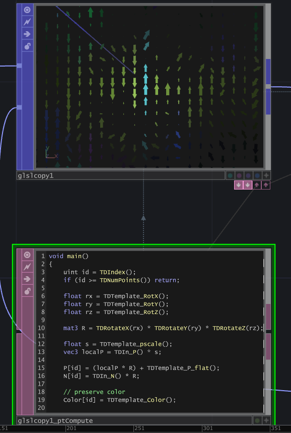
glslcopy1 is a GLSL Copy POP that instances a small arrow on every point of the field.
The copy shader reads from the template:
RotX
RotY
RotZ
pscale
P_flat
Color
The arrow mesh is scaled, rotated, and moved to the position of the point:
P[id] = (localP * R) + TDTemplate_P_flat();I use P_flat because the arrows need to remain legible as an oriented field. If they used the position with relief, the result would become more spatial, but also more confused.
3.5 glslcopy2
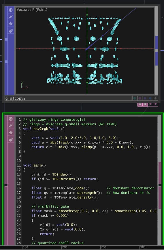
After the main field, I create a second layer of geometry with small rings.
First, I filter the points with group2:
density > 0.837Then delete2 keeps only those points. This filter exists because the rings work better as selective markers. If they appeared everywhere, they would cover the field instead of adding information to it.
glslcopy2 reads directly from the template attributes:
qdom
qstrength
density
In the network, I also have CHOPs connected as uniforms, such as uParams and uRingParams, but in the current ring shader code they are not declared or used. The ring shader is based only on the attributes of the field. So those parameters are inactive in this version, unless I later decide to use them to control ring scale, thresholds, or animation externally.
First, the shader calculates a visibility mask:
mask = smoothstep(0.2, 0.6, qstrength) * smoothstep(0.05, 0.2, density);Then it uses qdom to decide the radius of the ring:
shell = clamp(qdom, 1.0, 12.0);
r = 0.006 + 0.010 * sqrt(shell / 12.0);
The rings mark the points where a rational hierarchy is strong enough to stand out. The arrows show the local orientation of the bands; the rings show where a certain scale q emerges more clearly.
Finally, the ring branch passes through a Trail POP. Since the flux moves over time, the rings appear, shift, and leave a trace.
3.6 Final structure
In the end, the system overlays three readings of the same field.
The first GLSL shader calculates density, relief, color, and rational hierarchy.glslcopy1 transforms the gradient of the density into a field of arrows.glslcopy2 highlights the areas where a denominator q dominates.
The result is a visualization of the butterfly as a system of attributes. Every point contains a position in the flux / energy plane, a density, a scale, a direction, and a rational hierarchy. The final form is the result of how this data is calculated, filtered, and copied into geometry.
4. Conclusion
The core of this project is the reality that this mathematical structure exists independently of our observation, waiting for the right physical or computational parameters to make it visible.
Right now, my TouchDesigner network is just a real-time analytical shortcut, but the next step would be to push past this approximation by implementing a rigorous matrix diagonalization algorithm within GLSL to calculate the actual eigenvalues. Ultimately, this experiment connects back to my ongoing research into non-human signals and the limits of machine perception. I see our attempts to visualize what we cannot directly see or feel as a systematic way of expanding our frame of reference. Most importantly, it is a reminder that complex order is always present in the background, provided we have the specific computational tools and correct posture required to pay attention to it.
Bibliography
D. R. Hofstadter, “Energy Levels and Wave Functions of Bloch Electrons in Rational and Irrational Magnetic Fields,” Physical Review B 14, 2239–2249 (1976). https://doi.org/10.1103/PhysRevB.14.2239
J. Padgett and M. A. Seaberg, Struck by Genius: How a Brain Injury Made Me a Mathematical Marvel (Houghton Mifflin Harcourt, 2014). Background: “Jason Padgett,” Wikipedia, https://en.wikipedia.org/wiki/Jason_Padgett
P. G. Harper, “Single Band Motion of Conduction Electrons in a Uniform Magnetic Field,” Proceedings of the Physical Society A 68, 874 (1955). https://doi.org/10.1088/0370-1298/68/10/304
R. Peierls, “Zur Theorie des Diamagnetismus von Leitungselektronen,” Zeitschrift für Physik 80, 763–791 (1933). https://doi.org/10.1007/BF01342591
K. P. Nuckolls, M. G. Scheer, D. Wong, M. Oh, R. L. Lee, J. Herzog-Arbeitman, K. Watanabe, T. Taniguchi, B. Lian, and A. Yazdani, “Spectroscopy of the Fractal Hofstadter Energy Spectrum,” Nature 639, 342–347 (2025). https://doi.org/10.1038/s41586-024-08550-2. On the “undershot the magic angle” detail: Princeton Department of Physics, “Quantum Fractal Patterns Visualized,” Feb. 28, 2025, https://phy.princeton.edu/news/quantum-fractal-patterns-visualized (quote from co-author Dillon Wong).
X. Lu, B. Lian, G. Chaudhary, B. A. Piot, G. Romagnoli, K. Watanabe, T. Taniguchi, M. Poggio, A. H. MacDonald, B. A. Bernevig, and D. K. Efetov, “Multiple Flat Bands and Topological Hofstadter Butterfly in Twisted Bilayer Graphene Close to the Second Magic Angle,” Proceedings of the National Academy of Sciences 118, e2100006118 (2021). https://doi.org/10.1073/pnas.2100006118
G. H. Hardy and E. M. Wright, An Introduction to the Theory of Numbers, 6th ed. (Oxford University Press, 2008), Chapter 3, “Farey Series and a Theorem of Minkowski.”
G. H. Wannier, “A Result Not Dependent on Rationality for Bloch Electrons in a Magnetic Field,” Physica Status Solidi (b) 88, 757–765 (1978). https://doi.org/10.1002/pssb.2220880243
D. J. Thouless, M. Kohmoto, M. P. Nightingale, and M. den Nijs, “Quantized Hall Conductance in a Two-Dimensional Periodic Potential,” Physical Review Letters 49, 405–408 (1982). https://doi.org/10.1103/PhysRevLett.49.405
Code appendix: glsl_FIELD
// hofstadter butterfly field
// lightweight analytical approximation for real-time visualization
//
// this shader does not diagonalize the harper-hofstadter hamiltonian.
// it uses rational approximations p/q and simplified band curves to build
// a visual density field in flux / energy space.
//
// outputs:
// p, p_flat, density, pscale, color, rotx, roty, rotz, gmag, qdom, qstrength
//
// uniforms:
// uparams  = (maxq, detail, time, brightness)
// uparams2 = (bandcontrast, unused, fluxspeed, unused)
// uparams3 = (heightscale, unused, unused, unused)

const float TWO_PI = 6.28318530718;
const int MAX_Q_CAP = 128;

uniform vec4 uParams[1];
uniform vec4 uParams2[1];
uniform vec4 uParams3[1];

vec3 hsv2rgb(vec3 c)
{
    vec4 k = vec4(1.0, 2.0 / 3.0, 1.0 / 3.0, 3.0);
    vec3 p = abs(fract(c.xxx + k.xyz) * 6.0 - k.www);
    return c.z * mix(k.xxx, clamp(p - k.xxx, 0.0, 1.0), c.y);
}

float toneMapDensity(float rawDensity, float brightness, float contrast)
{
    brightness = max(brightness, 0.0);
    contrast = max(contrast, 0.001);

    float mapped = 1.0 - exp(-rawDensity * brightness);
    mapped = pow(mapped, contrast);

    return clamp(mapped, 0.0, 1.0);
}

float simplifiedBandEnergy(float phi, int bandIndex)
{
    float k = float(bandIndex);
    return 2.0 * cos(TWO_PI * phi * k);
}

float approximationQuality(float flux, float phi, float q)
{
    flux = fract(flux);

    float dist = abs(flux - phi);
    dist = min(dist, 1.0 - dist);

    return 1.0 / (1.0 + dist * q * q);
}

void computeHofstadterDensity(
    float flux,
    float energy,
    int maxQ,
    float detail,
    out float density,
    out float dominantQ,
    out float qStrength
)
{
    flux = fract(flux);
    detail = clamp(detail, 0.0, 1.0);
    maxQ = max(1, min(maxQ, MAX_Q_CAP - 1));

    float totalDensity = 0.0;
    float qContributions[MAX_Q_CAP];

    for (int i = 0; i < MAX_Q_CAP; i++)
    {
        qContributions[i] = 0.0;
    }

    float sigma = mix(0.12, 0.04, detail);

    for (int q = 1; q < MAX_Q_CAP; q++)
    {
        if (q > maxQ)
        {
            break;
        }

        float qf = float(q);

        int p = int(flux * qf + 0.5);
        p = max(0, min(p, q));

        float phi = float(p) / qf;
        float quality = approximationQuality(flux, phi, qf);

        float qContribution = 0.0;

        for (int band = 0; band < MAX_Q_CAP; band++)
        {
            if (band >= q)
            {
                break;
            }

            float bandEnergy = simplifiedBandEnergy(phi, band);
            float energyDist = energy - bandEnergy;

            float gaussian = exp(
                -(energyDist * energyDist) / (2.0 * sigma * sigma)
            );

            float contribution = gaussian * quality / sqrt(qf);

            qContribution += contribution;
            totalDensity += contribution;
        }

        qContributions[q] = qContribution;
    }

    float maxContribution = 0.0;
    float bestQ = 1.0;

    for (int q = 1; q < MAX_Q_CAP; q++)
    {
        if (q > maxQ)
        {
            break;
        }

        if (qContributions[q] > maxContribution)
        {
            maxContribution = qContributions[q];
            bestQ = float(q);
        }
    }

    float dominance = 0.0;

    if (totalDensity > 1e-8)
    {
        dominance = clamp(maxContribution / totalDensity, 0.0, 1.0);
    }

    density = totalDensity;
    dominantQ = bestQ;
    qStrength = dominance;
}

void main()
{
    uint id = TDIndex();

    if (id >= TDNumElements())
    {
        return;
    }

    float fluxInput = TDIn_flux(0, id);
    float energyInput = TDIn_energy(0, id);

    int maxQ = int(uParams[0].x + 0.5);
    float detail = uParams[0].y;
    float timeVal = uParams[0].z;
    float brightness = uParams[0].w;

    float bandContrast = uParams2[0].x;
    float fluxSpeed = uParams2[0].z;

    float heightScale = uParams3[0].x;

    maxQ = max(1, min(maxQ, MAX_Q_CAP - 1));
    detail = clamp(detail, 0.0, 1.0);

    float flux = fract(fluxInput + timeVal * fluxSpeed);
    float energy = energyInput;

    float rawDensity;
    float qDom;
    float qStr;

    computeHofstadterDensity(
        flux,
        energy,
        maxQ,
        detail,
        rawDensity,
        qDom,
        qStr
    );

    float densityMapped = toneMapDensity(rawDensity, brightness, bandContrast);
    densityMapped = smoothstep(0.02, 0.98, densityMapped);

    density[id] = densityMapped;
    qdom[id] = qDom;
    qstrength[id] = qStr;

    float eps = 0.003;

    float dTmp;
    float qTmp;
    float qsTmp;

    computeHofstadterDensity(
        flux + eps,
        energy,
        maxQ,
        detail,
        dTmp,
        qTmp,
        qsTmp
    );
    float dxPlus = toneMapDensity(dTmp, brightness, bandContrast);

    computeHofstadterDensity(
        flux - eps,
        energy,
        maxQ,
        detail,
        dTmp,
        qTmp,
        qsTmp
    );
    float dxMinus = toneMapDensity(dTmp, brightness, bandContrast);

    computeHofstadterDensity(
        flux,
        energy + eps,
        maxQ,
        detail,
        dTmp,
        qTmp,
        qsTmp
    );
    float dyPlus = toneMapDensity(dTmp, brightness, bandContrast);

    computeHofstadterDensity(
        flux,
        energy - eps,
        maxQ,
        detail,
        dTmp,
        qTmp,
        qsTmp
    );
    float dyMinus = toneMapDensity(dTmp, brightness, bandContrast);

    float gx = (dxPlus - dxMinus) / (2.0 * eps);
    float gy = (dyPlus - dyMinus) / (2.0 * eps);

    float gradMag = length(vec2(gx, gy));
    float gmagNorm = clamp(gradMag * 3.0, 0.0, 1.0);

    gmag[id] = gmagNorm;

    float angle = atan(gx, -gy);

    float snapStrength = smoothstep(0.05, 0.25, densityMapped);
    float angleSteps = 12.0;
    float angleStepSize = TWO_PI / angleSteps;

    float angleSnapped = round(angle / angleStepSize) * angleStepSize;
    angle = mix(angle, angleSnapped, snapStrength);

    RotZ[id] = angle;
    RotX[id] = -clamp(gmagNorm * 0.5, 0.0, 0.5) * snapStrength;
    RotY[id] = 0.0;

    float avgNeighbor = 0.25 * (dxPlus + dxMinus + dyPlus + dyMinus);

    float relief = densityMapped - avgNeighbor;
    relief = clamp(relief * 10.0, -1.0, 1.0);
    relief = max(relief, 0.0);
    relief = smoothstep(0.0, 1.0, relief);
    relief *= snapStrength;

    vec3 pFlat = TDIn_P(0, id);
    vec3 pRelief = pFlat;

    pRelief.z += relief * heightScale;

    P[id] = pRelief;
    P_flat[id] = pFlat;

    float qNormalized = (qDom - 1.0) / max(1.0, float(maxQ - 1));
    qNormalized = clamp(qNormalized, 0.0, 1.0);

    float hue = fract(qNormalized * 0.75);
    float sat = mix(0.15, 0.95, qStr * snapStrength);
    float val = pow(densityMapped, 0.6);

    vec3 rgb = hsv2rgb(vec3(hue, sat, val));
    Color[id] = vec4(rgb, 1.0);

    float baseScale = 0.008;
    float scaleRange = 0.12;

    float ps = baseScale + scaleRange * pow(densityMapped, 1.2);
    ps *= mix(0.7, 1.3, relief);

    pscale[id] = clamp(ps, 0.001, 0.3);
}